
A floor feels solid because its structure quietly distributes every footstep, bookshelf, partition wall, and vibration into beams, columns, and foundations. Yet before concrete is poured or steel is erected, an engineer must predict how that load will travel and where the structure may bend, crack, buckle, or vibrate.
For a simple beam, hand calculations can reveal a great deal. For a hospital floor with irregular openings, a long-span roof, or a high-rise exposed to wind and earthquake loading, the interacting parts quickly become too numerous for a single closed-form equation.
Finite element analysis (FEA) makes those complex predictions manageable. It does not replace structural judgement; it converts a physical structure into a mathematical model that can be solved systematically.
The algorithms behind FEA explain both its extraordinary usefulness and its most serious danger: a computer can solve the wrong model with remarkable efficiency.
🧩 Finite Element Analysis as Controlled Approximation
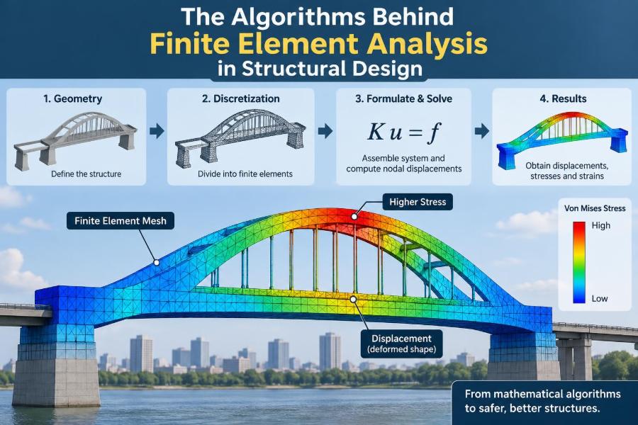
FEA divides a continuous body or structural system into many small, connected pieces called elements. The elements meet at points called nodes, where the program tracks unknown movements such as translations and rotations.
Rather than finding the exact displacement at every point in a slab or frame, the method approximates the response from values at the nodes. More elements can generally represent local behavior better, but only when their formulation, shape, and restraints are appropriate.
🏗️ Why Structures Need Numerical Models
Classical structural analysis works elegantly for idealized beams, trusses, and plates with regular geometry and familiar boundary conditions. Real buildings combine all of these, often with transfer levels, cores, openings, offsets, diaphragms, and nonlinear supports.
FEA lets the engineer represent load paths across that connected system. Its value is not merely handling a larger number of members; it reveals how stiffness changes redirect forces, sometimes in ways that member-by-member calculations can miss.
📐 The Physical Problem Before the Mathematics
Every analysis begins with equilibrium, compatibility, and material behavior. Equilibrium requires forces and moments to balance. Compatibility requires connected points to move consistently. Constitutive behavior relates stress to strain, such as the elastic relationship represented by Young’s modulus.
An algorithm cannot decide which physical behavior matters. The engineer must decide whether a connection acts pinned or fixed, whether a wall participates in lateral resistance, and whether cracking, yielding, contact, or large movement must be considered.
🔢 Degrees of Freedom Define the Unknowns
A degree of freedom (DOF) is an independent nodal movement. A planar truss node may have horizontal and vertical translation. A three-dimensional frame node commonly has three translations and three rotations.
Collecting all unknown nodal movements gives a displacement vector, commonly written as {u}. The number of DOFs controls the size of the computational problem. It also exposes modelling errors: an unrestrained rigid-body movement produces a mechanism rather than a stable structural model.
🧱 Elements Are Mathematical, Not Physical Blocks
A beam element represents axial, shear, bending, and sometimes torsional behavior along a line. A shell element can represent both in-plane membrane action and out-of-plane bending. Solid elements represent three-dimensional stress states within a volume.
The element is an idealization, not a miniature piece of construction. Modelling a deep transfer member as a line beam may hide important shear and strut-and-tie behavior; modelling every steel member as solids may create a costly model without a better design answer.
🕸️ Shape Functions Interpolate Movement
Within each element, shape functions estimate displacement between nodes. For a basic bar element, displacement may vary linearly from one end to the other. More advanced elements use higher-order functions and can represent curvature or complex field variation more efficiently.
Strain follows from displacement gradients, and stress follows from strain through the material law. This chain—nodal movement to interpolated movement to strain to stress—is the core computational idea behind most structural finite elements.
⚙️ From Material Stiffness to the Element Matrix
Each element produces an equation linking its nodal forces and displacements: {f}e = [k]e{u}e. The matrix [k]e is the element stiffness matrix.
Its entries express a practical question: if one nodal movement is imposed, what resisting force or moment appears at this and neighboring DOFs? Geometry, section properties, material stiffness, length, and element theory all affect the answer.
🧮 Numerical Integration Makes Complex Elements Work
For many elements, especially shells and solids, stiffness terms involve integrals that are inconvenient or impossible to evaluate by hand for every geometry. Software usually evaluates them using numerical quadrature, often called Gauss integration.
The program samples the element at selected integration points and combines those values using weights. Too few points may miss bending or nonlinear behavior; unsuitable integration choices can also introduce artificial flexibility or spurious deformation patterns.
🧷 Coordinate Transformations Align Local Behavior
An element is easiest to formulate in its own local axes: along a beam, across a shell, or through a thickness. A building model, however, is assembled in one global coordinate system.
Transformation matrices rotate and translate local stiffness and load quantities into global directions. Incorrect local-axis orientation is a common source of puzzling results, particularly for shells, releases, eccentricities, and directional loads.
🧩 Assembly Builds the Global Stiffness Matrix
Assembly places every element matrix into a much larger global matrix according to node numbering and DOF connectivity. Contributions from elements meeting at a node are added together, exactly as their physical stiffnesses act together.
The resulting equation is commonly written as [K]{u} = {F}, where [K] is global stiffness and {F} is the global load vector. This compact equation can represent thousands or millions of unknowns.
🔒 Boundary Conditions Prevent a Mathematical Collapse
Supports, restraints, prescribed displacements, and connection releases are boundary conditions. They tell the model which movements are prevented, allowed, or imposed.
A structure resting freely in space has no unique static solution: it can translate and rotate without strain. Conversely, over-restraint can create artificial forces. A model that “runs” is not necessarily a model with physically credible support conditions.
⚖️ Loads Become Equivalent Nodal Forces
Analysis software ultimately needs loads expressed consistently with its DOFs. A distributed beam load, pressure on a slab, thermal strain, settlement, or imposed acceleration may be converted into equivalent nodal forces or handled through an appropriate element load formulation.
Load direction deserves close attention. Gravity loads usually act globally downward, while wind pressure may be normal to a changing surface, and live-load patterns may need several arrangements to capture the critical effect.
🧠 Linear Static Analysis Solves the Familiar Equation
In linear static analysis, stiffness is assumed constant, displacements are small, and load effects scale proportionally. Double a load and the calculated displacement, force, and elastic stress double.
This is often appropriate for preliminary work and many service-level checks. It is fast, interpretable, and useful—but it cannot by itself capture yielding, cracking redistribution, cable slackening, contact separation, or instability after stiffness changes.
🚀 Sparse Solvers Make Large Models Practical
Although [K] can be enormous, most entries are zero because an element connects only nearby nodes. Such matrices are called sparse.
Modern solvers store and operate mainly on nonzero entries. Direct methods factor the matrix efficiently and robustly; iterative methods repeatedly improve an estimated solution and can be attractive for very large problems. Solver choice affects speed and memory, not the need for sound engineering assumptions.
🔁 Iterative Algorithms Chase Nonlinear Equilibrium
Nonlinear analysis is required when stiffness changes with deformation, material response, or contact state. The governing relation is no longer one fixed matrix equation.
A common approach applies load in increments, estimates a displacement change, updates stiffness, and repeats until internal and external forces balance within selected tolerances. Newton-Raphson-type procedures use a tangent stiffness to correct the estimate efficiently near equilibrium.
📉 Material Nonlinearity Models Yielding and Cracking
Steel may yield, concrete may crack in tension and crush in compression, and reinforcing steel may enter a nonlinear stress-strain range. These effects alter stiffness and redistribute force through the system.
Material models require careful calibration and interpretation. A nonlinear concrete result is not automatically more realistic than a linear model; uncertainty in cracking, reinforcement representation, confinement, and load history can dominate the apparent precision.
📐 Geometric Nonlinearity Captures Changing Shape
Geometric nonlinearity accounts for equilibrium on the deformed shape. Axial force can magnify lateral displacement, the familiar P-Delta effect, and slender members may lose stiffness as they deflect.
For a tall frame under gravity and lateral load, second-order effects can materially change drift and member actions. For a compact, well-braced low-rise component, they may be negligible. The decision should follow expected deformation and code-required stability checks.
🫱 Contact, Gaps, and Compression-Only Supports
Some interfaces transmit compression but not tension, such as a bearing that can lift off, soil idealized as compression-only springs, or a member with a gap. Contact algorithms must determine whether the interface is open, closed, sticking, or sliding.
These status changes make the problem nonlinear. Simplifying them as permanently connected can create fictitious tensile forces; simplifying them as absent can remove real load transfer. The correct abstraction depends on the design question.
🧱 Meshing Balances Resolution and Reliability
A mesh is the arrangement and size of elements. Fine mesh is useful near openings, concentrated loads, supports, re-entrant corners, and abrupt stiffness changes, where response gradients are high.
Uniformly making every element tiny is not a universal solution. It increases run time, can worsen conditioning, and may report meaningless local stress spikes. A good mesh follows structural behavior and is tested by refinement.
🔍 Mesh Convergence Tests the Approximation
Mesh convergence means comparing results as the mesh is refined. Global outputs such as total reaction, midspan deflection, natural period, or design section force should approach a stable value.
Do not expect every peak stress to converge. An ideal point load, perfectly sharp corner, or fixed boundary can create a mathematical singularity, where computed stress rises as elements become smaller. Design should use averaged, distributed, or code-consistent quantities away from the singular point.
🚨 Singularities Are Warnings, Not Design Forces
A vivid contour plot can show an extreme red spot at a point support or sharp opening corner. That may indicate a genuine detailing concern, but the highest numerical value may not be a physically usable stress.
Ask what exists in construction: a bearing plate, weld length, reinforcement development zone, fillet radius, or finite contact area. Model or assess that real load-distribution mechanism instead of designing solely to a single nodal peak.
🌊 Dynamic Analysis Adds Mass and Time
When loading changes rapidly, inertia and damping matter. The equation becomes [M]{a} + [C]{v} + [K]{u} = {F}(t), where mass, damping, acceleration, velocity, and time-varying load enter the response.
This framework supports vibration assessment, machinery response, footfall studies, blast idealizations, wind response, and earthquake analysis. The reliability of the result depends strongly on mass distribution, stiffness assumptions, damping treatment, and the chosen loading representation.
🎵 Modal Analysis Finds Natural Vibration Patterns
Modal analysis solves an eigenvalue problem to find natural frequencies and mode shapes. A mode shape is a preferred pattern in which the structure can vibrate, not a literal load case or final deformed building.
Low-frequency modes often govern global lateral behavior, while higher modes can matter near irregularities or in acceleration-sensitive structures. Reviewing mode shapes is a powerful diagnostic: unexpected twisting can reveal eccentric stiffness, mass, or diaphragm assumptions.
🌐 Response Spectrum and Time-History Methods
Response spectrum analysis combines modal responses using a specified spectral demand. It is efficient for many seismic design applications but relies on assumptions about modal combination, directionality, damping, and scaling required by the governing design framework.
Time-history analysis applies acceleration or force records through time and integrates the equations step by step. It can represent sequencing and nonlinear response in greater detail, but record selection, baseline treatment, timestep choice, and interpretation demand substantial care.
🏢 Diaphragms Control the Building-Wide Load Path
Floor slabs often distribute lateral loads to walls and frames as diaphragms. A rigid diaphragm idealization may be suitable for a compact, stiff floor; a semi-rigid shell model may be needed where slabs are long, flexible, perforated, or heavily discontinuous.
The choice affects torsion, collector forces, wall reactions, and drift distribution. It should be based on comparative stiffness and geometry, not simply on whichever software option is fastest to select.
🧭 Verification and Validation Answer Different Questions
Verification asks whether the mathematical model and software setup solve the intended equations correctly. Useful checks include reaction balance, hand-calculation benchmarks, symmetry, deformed-shape review, and simplified submodels.
Validation asks whether those equations and assumptions represent the actual structure adequately. It may involve comparing known behavior, test information where available, construction details, monitoring data, and engineering experience. A verified model can still be invalid for its intended decision.
🧪 A Simple Portal Frame as a Diagnostic Example
Consider a hypothetical single-bay steel portal frame under vertical roof load and lateral wind. Before examining colorful diagrams, predict the behavior: gravity should flow through rafters into columns, wind should create sway, and fixed bases should develop moments.
Now check the model. Do vertical reactions equal the applied gravity load? Does reversing wind reverse sway? If a base is released, do base moments reduce and drift increase? These simple expectations are often more revealing than a dense output report.
🛑 Common Modelling Mistakes That Produce Convincing Errors
- Duplicate or disconnected nodes: members look connected but do not transfer force.
- Unintended releases: a frame becomes a mechanism or loses moment continuity.
- Misassigned section properties: stiffness, weight, and force distribution become wrong together.
- Incorrect units: a model may solve without warning while deflections become implausible.
- Ignoring self-weight or mass: gravity and dynamic results no longer represent the building.
- Reading contours without scale: local artifacts are mistaken for governing design demands.
Most of these errors are prevented by deliberate review, not by purchasing more sophisticated software.
📋 A Practical Analysis Workflow
- Define the design questions: strength, serviceability, stability, vibration, or construction-stage behavior.
- Establish the intended load path and choose suitable idealizations.
- Build geometry, connectivity, supports, properties, loads, and combinations with consistent units.
- Run simple checks before advanced analysis: reactions, deformed shape, member forces, and modal behavior.
- Refine the model only where the decision requires greater fidelity.
- Convert analysis actions into code-compliant member, connection, foundation, and detailing checks.
This sequence prevents a detailed model from becoming an elaborate answer to an undefined question.
🧑💼 Engineering Judgement Remains Outside the Solver
Software can factor a matrix, iterate to equilibrium, and display stress fields. It cannot independently determine whether a load combination is complete, whether a construction joint changes continuity, or whether a plausible-looking deformation conflicts with how the structure will actually be built.
Experienced engineers use algorithms as transparent tools. They predict broad behavior first, examine results at several scales, and investigate discrepancies rather than selecting the output that appears most convenient.
🧠 The Core Principle: Model the Behavior You Need to Know
The most useful FEA model is not necessarily the largest or most detailed. It is the simplest model that represents the behavior governing the decision, while making its assumptions visible and checkable.
Elements, matrices, numerical integration, and solvers provide the machinery. Boundary conditions, material assumptions, mesh choices, and validation determine whether that machinery is describing the real structural problem. Finite element analysis earns trust when numerical sophistication is matched by physical understanding and independent checks.
Learn the algorithms well enough to question them, and use structural intuition well enough to recognize when the model is asking for a better question. 🏗️📐🔍