The previous discussion was focused on the source of loadings, i.e., environmental, functional, construction, and terrorist activity. Loadings are also characterized by attributes, which relate to properties of the loads. Table 1.3 lists the most relevant attributes and their possible values.

Duration relates to the time period over which the loading is applied. Long-term loads, such as self-weight are referred to as dead loads. Loads whose magnitude or location changes are called temporary loads. Examples of temporary loads are the weight of vehicles crossing a bridge, stored items in buildings, wind and seismic loads, and construction loads.

Most loads are represented as being applied over a finite area. For example, a line of trucks is represented with an equivalent uniformly distributed load. However, there are cases where the loaded area is small, and it is more convenient to treat the load as being concentrated at a particular point. A member partially supported by cables such as a cable-stayed girder is an example of concentrated loading.

Temporal distribution refers to the rate of change of the magnitude of the temporary loading with time. An impulsive load is characterized by a rapid increase over a very short duration and then a drop off. Figure 1.9 illustrates this case. Examples are forces due to collisions, dropped masses, brittle fracture material failures, and slamming action due to waves breaking on a structure. Cyclic loading alternates in direction (+ and ) and the period may change for successive cycles. The limiting case of cyclic loading is harmonic excitation where the amplitude and period are constant. Seismic excitation is cyclic. Rotating machinery such as printing presses, electric generators, and turbines produce harmonic excitation on their supports when they are not properly balanced. Quasi-static loading is characterized by a relatively slow build

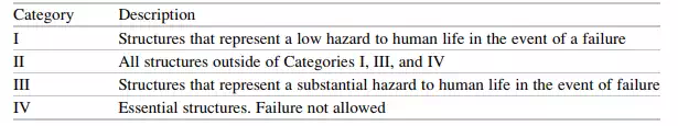
Table 1.4 Occupancy categories

up of magnitude, reaching essentially a steady state. Because they are applied slowly, there is no appreciable dynamic amplification and the structure responds as if the load was a static load. Steady winds are treated as quasi-static; wind gusts are impulsive. Wind may also produce a periodic loading resulting from vortex shedding. We discuss this phenomenon later in this section.

The design life of a structure is that time period over which the structure is expected to function without any loss in operational capacity. Civil structures have long design lives vs. other structures such as motorcars, airplanes, and computers. A typical building structure can last several centuries. Bridges are exposed to more severe environmental actions, and tend to last a shorter period, say 50–75 years. The current design philosophy is to extend the useful life of bridges to at least 100 years. The Millau viaduct shown in Fig. 1.8 is intended to function at its full design capacity for at least 125 years.

Given that the natural environment varies continuously, the structural engineer is faced with a difficult problem: the most critical natural event, such as a windstorm or an earthquake that is likely to occur during the design life of the structure located at a particular site needs to be identified. To handle this problem, natural events are modeled as stochastic processes. The data for a particular event, say wind velocity at location x, is arranged according to return period which can be interpreted as the average time interval between occurrences of the event. One speaks of the 10-year wind, the 50-year wind, the 100-year wind, etc. Government agencies have compiled this data, which is incorporated in design codes. Given the design life and the value of return period chosen for the structure, the probability of the structure experiencing the chosen event is estimated as the ratio of the design life to the return period. For example, a building with a 50-year design life has a 50 % chance of experiencing the 100-year event during its lifetime. Typical design return periods are 50 years for wind loads and between 500 and 2,500 years for severe seismic loads.

Specifying a loading having a higher return period reduces the probability of occurrence of that load intensity over the design life. Another strategy for establishing design loads associated with uncertain natural events is to increase the load magnitude according to the importance of the structure. Importance is related to the nature of occupancy of the structure. In ASCE Standards 7-05 [8], four occupancy categories are defined using the potential hazard to human life in the event of a failure as a basis. They are listed in Table 1.4 for reference.

The factor used to increase the loading is called the importance factor, and denoted by I. Table 1.5 lists the values of I recommended by ASCE 7-05 [8] for each category and type of loading.

Table 1.5 Values of I

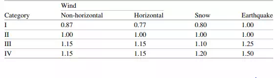
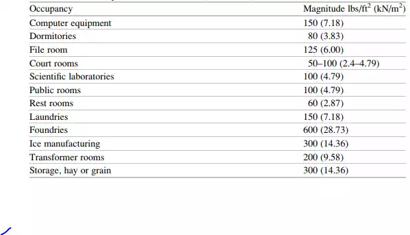
Table 1.6 Uniformly distributed live loads (ASCE 7-05)

For example, one increases the earthquake loading by 50 % for an essential structure (category 4).

Gravity Live Loads

Gravitational loads are the dominant loads for bridges and low-rise buildings located in areas where the seismic activity is moderate. They act in the downward vertical direction and are generally a combination of fixed (dead) and temporary (live) loads. The dead load is due to the weight of the construction materials and permanently fixed equipment incorporated into the structure. As mentioned earlier, temporary live loads depend on the function of the structure. Typical values of live loads for buildings are listed in Table 1.6. A reasonable estimate of live load for office/residential facilities is 100 lbs/ft2 (4.8 kN/m2 ). Industrial facilities have higher live loadings, ranging up to 600 lbs/ft2 for foundries.

Live loading for bridges is specified in terms of standard truck loads. In the USA, bridge loads are defined by the American Association of State Highway and Transportation Officials (AASHTO). They consist of a combination of the Design truck or tandem, and Design lane load.

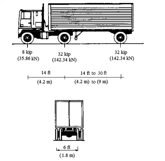
Fig. 1.10 Characteristics of the AASHTO Design Truck

The design truck loading has a total weight of 72 kip (323 kN), with a variable axle spacing is shown in Fig. 1.10. The design tandem shall consist of a pair of 25 kip (112 kN) axles spaced 4 ft (1.2 m) apart. The transverse spacing of wheels shall be taken as 6 ft (1.83 m). The design lane load shall consist of a load of 0.64 kip/ft2 (30.64 kN/m2 ) uniformly distributed in the longitudinal direction and uniformly distributed over a 10 ft (3 m) width in the transverse direction.