We will look at the development of the matrix structural analysis method for the simple case of a structure made only out of truss elements that can only deform in one direction. This will allow us to get a taste of how matrix structural analysis works without having to learn about all of the details and complexities that are present in beam and frame systems. As we will see, since we have only one-dimensional truss elements, each node in the system only has one possible degree of freedom (translation along the axis of the structural members). In previous stiffness methods, each degree of freedom was dealt with separately. For example, in the slope-deflection method, we ended up with one equation for each degree of freedom. Then we had to solve for the unknown deflections and rotations by solving the system of equations.
In matrix structural analysis, we will end up with the same equations. But we will construct those equations using matrices that represent each element stiffness. Putting these stiffness matrices together, we will be able to construct a large matrix for the entire structure, that represents all of the equations that we had previously in the slope-deflection method. Since all of our equations will be in matrix form, we can take advantage of matrix methods to solve the system of equations and determine all of the unknown deflections and forces. Computers are well-adapted to solve such matrix problems.
The One-Dimensional Truss Element
Recall that the deformation of a truss element may be found using the following equation:
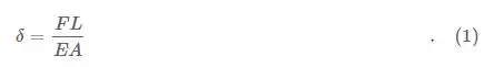
where δδ is the axial deformation, FF is the axial force in the truss element, LL is the length of the element, EE is the Young’s modulus, and AA is the cross-sectional area of the element. This equation may be rearranged to find the following relationship between axial force and axial deformation:
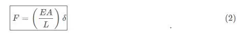
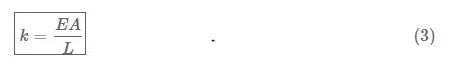
The term that is multiplied by the deformation to get the force is the axial stiffness:
With this background, we can look at the behaviour of a one-dimensional truss element as shown in Figure 11.1. This truss element has a constant Young’s modulus EE and cross-sectional area AA. It has two ends, which we can consider to be connected to two separate nodes in our structure, one labelled ‘1’ and one labelled ‘2’ as shown in the figure. We can represent the complete behaviour of this entire element through the force and displacement of the two nodes. The force at node 1 is labelled Fx1Fx1 and the force at node two is labelled Fx2Fx2. Likewise, the displacement of node 1 (relative to its initial position) is labelled Δx1Δx1 and the displacement of node two is labelled Δx2Δx2.
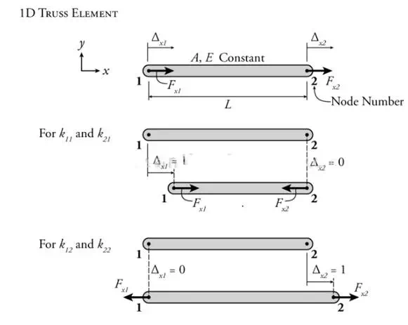
Figure 11.1: One-Dimensional Truss Element
We can relate the forces to the displacements at the two ends of the member using the stiffness term from equation (3)(3); however, we need to relate the end displacement to the bar deformation (these are not the same thing). For, example, if both the left and right sides move by 1.0 unit positive (to the right), then the entire bar moves to the right as a rigid body, neither expanding or contracting, so the deformation would be zero. The deformation can be related to the end node displacements as follows:

So, the total internal axial force in the bar is equal to:
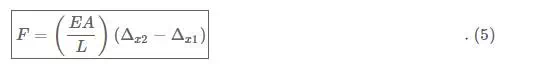
Due to horizontal equilibrium, Fx1=−Fx2Fx1=−Fx2. The magnitude of these external forces is equal to the internal force in the truss element. If the internal force from equation (5)(5) is positive, the bar is in tension, so the force on the left (Fx1Fx1) must point to the left (negative), and the force on the right (Fx2Fx2) must point to the right (positive). So:
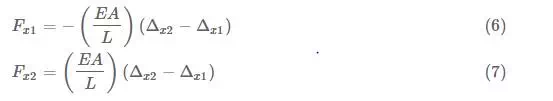
These two equations define the force/deflection behaviour of the truss at both nodes simultaneously. They are only a function of displacements of the nodes (the nodal displacements) and the forces applied to the nodes (the nodal forces).
We can easily express these two equations in a matrix form as follows:
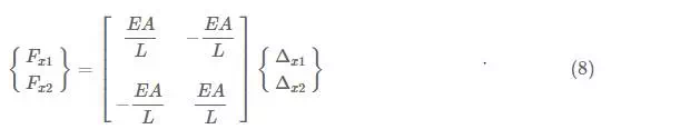
where the matrix on the left of the equal sign is called the force vector, the large central matrix is called the stiffness matrixand the smaller matrix on the right with the displacements is called the displacement vector. The term vector just means a matrix with only one column. If we multiply the large central matrix by the vector of displacements on the right, we get:
which are the same as equations (6)(6) and (7)(7). This matrix equation constitutes a complete model for the behaviour of a one-dimensional truss element. The large matrix in the middle is called the stiffness matrix of the element because it contains all of the stiffness terms. It contains the most important information for the model, and it is useful to think about it as a separate element:
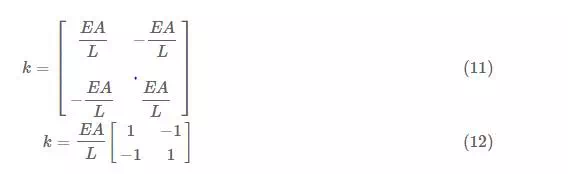
This is the stiffness matrix of a one-dimensional truss element. Other types of elements have different types of stiffness matrices. For a truss element in 2D space, we would need to take into account two extra degrees of freedom per node as well as the rotation of the element in space. Beam elements that include axial force and bending deformations are more complex still. For real physical systems, stiffness matrices are always square and symmetric about the diagonal axis of the matrix.
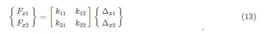
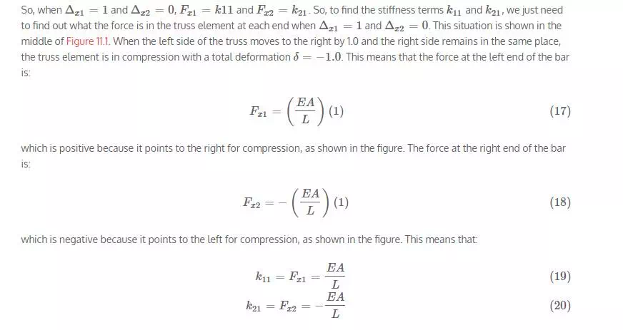
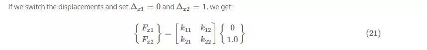
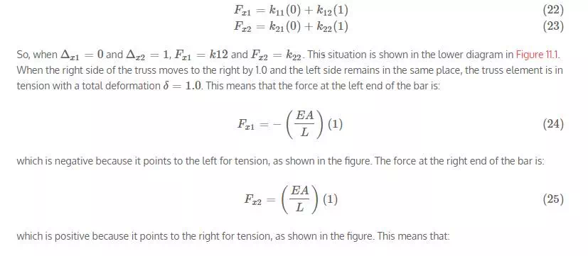
Another way to think about the construction of a stiffness matrix is to find the forces at either end of the element if the element experiences a unit deformation at each end (separately). This works because the stiffness is defined as the force per unit deformation. If we don’t know the stiffness matrix, we can figure it out by first starting with the general form of the stiffness matrix for our element:

So let’s individually set each displacement to 1.0 while setting the other to zero to calculate the stiffness terms. This process is shown in Figure 11.1. If we set Δx1=1Δx1=1 and Δx2=0Δx2=0, we get:
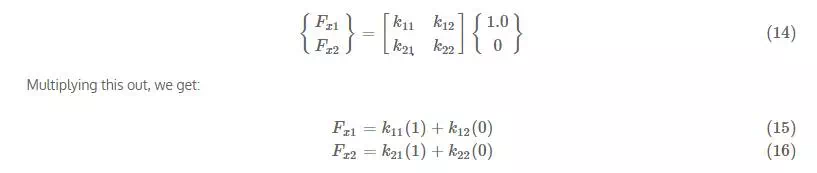
Multiplying this out, we get:
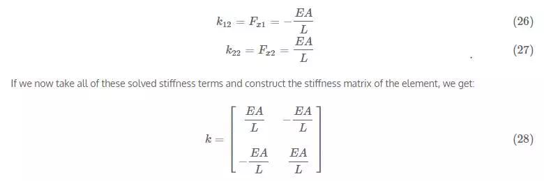
which is the same stiffness matrix that we derived previously in equation
Assembling the Full Stiffness Matrix
If we have a structural analysis problem with multiple one-dimensional truss elements, we must first define the stiffness matrices for each individual element as described in the previous section. After we define the stiffness matrix for each element, we must combine all of the elements together to form on global stiffness matrix for the entire problem. This matrix defines all of the interconnections between the elements and includes all of the information related to the stiffness of each element for each degree-of-freedom.
The resulting global stiffness matrix is put into an equation with the global nodal force vector (which contains all of the forces for each node in each DOF) and the global nodal displacement vector (which contains all of the displacements of each node in each DOF) to get a global system of equations for the entire problem with the following form:
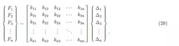
Solving for Nodal Forces and Displacements
Once the stiffness matrix is formed, the full system of equations in the form shown in equation (29)(29) may be solved. At each nodal DOF (each row), we must either know the external force or the nodal deflection. Then, we can solve only those rows where we don’t know the deflection. Once we have all of the nodal deflections, we can solve for the nodal forces. Then, using the individual element stiffness matrices, we can solve for the internal force in each element.
There are numerous different computer algorithms that may be used to solve the matrix of equations, but these are outside the scope of this book.
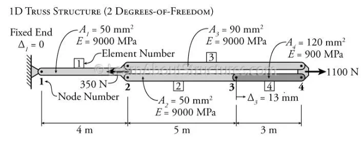
Example
The full process for a matrix structural analysis for a one dimensional truss will be demonstrated using the simple example shown in Figure 11.2. This is a one dimensional structure, meaning that all of the nodes are only permitted to move in one direction. This structure consists of four different truss elements which are numbered one through four as shown in the figure. These elements are connected at four different nodes, also numbered one through four as shown. The left end of the structure, at node 1 is restrained and cannot move. Nodes 2 and 4 have external loads, and Node 3 has an imposed displacement of 13mm13mm to the right (positive).