First, it should be clarified that one should not get confused with the real body and its mathematical idealization. Modeling is all about idealizations that lead to predictions that are close to observations. To illustrate, the earth and the sun are assumed as point masses when one is interested in planetary motion. The same earth is assumed as a rigid sphere if one is interested in studying the eclipse. These assumptions are made to make the resulting problem tractable without losing on the required accuracy. In the same sprit, the all material responses, some amount of mechanical energy is converted into other forms of energy. However, in some cases, this loss in the mechanical energy is small that it can be idealized as having no loss, i.e., a non-dissipative process.

Non-dissipative response

A response is said to be non-dissipative if there is no conversion of mechanical energy to other forms of energy, namely heat energy. Commonly, a material responding in this fashion is said to be elastic. The common definitions of elastic response,

• If the body’s original size and shape can be recovered on unloading, the loading process is said to be elastic.
• Processes in which the state of stress depends only on the current strain, is said to be elastic.

The first definition is of little use, because it requires one to do a complimentary process (unloading) to decide on whether the process that needs to be classified as being elastic. The second definition, though useful for deciding on the variables in the constitutive relation, it also requires one to do a complimentary process (unload and load again) to decide on whether the first process is elastic. The definition based on thermodynamics does not suffer from this drawback. In chapter 6 we provide examples where these three definitions are not equivalent. However, many processes (approximately) satisfy all the three definitions.

This class of processes also proceeds through thermodynamically equilibrated states. That is, if the body is isolated at any instant of loading (or displacement) then the stress, displacement, internal energy, entropy do not change with time.

Ideal gas, a fluid is the best example of a material that responds in a non-dissipative manner. Metals up to a certain stress level, called the yield stress, are also idealized as responding in a non dissipative manner. Thus, the notion that only solids respond in a non-dissipative manner is not correct.

Thus, for these non-dissipative, thermodynamically equilibrated processes the Cauchy stress and the deformation gradient can in general be related through an implicit function. That is, for isotropic materials (see chapter 6 for when a material is said to be isotropic), f(σ,F) = 0. However, in classical elasticity it is customary to assume that Cauchy stress in a isotropic material is a function of the deformation gradient, σ =  (F). On requiring the restriction⁶ due to objectivity and second law of thermodynamics to hold, it can be shown that if σ =  (F), then

(1.16)

where ψ_R =  _R(J₁,J₂,J₃) is the Helmoltz free energy defined per unit volume in the reference configuration, also called as the stored energy, B = FF^t and J ₁ = tr(B), J₂ = tr(B^–1), J ₃ = . When the components of the displacement gradient is small, then (1.16) reduces to,

(1.17)

on neglecting the higher powers of the Lagrangian displacement gradient and where λ and μ are called as the Lamè constants. The equation (1.17) is the famous Hooke’s law for isotropic materials. In this course Hooke’s law is the constitutive equation that we shall be using to solve boundary value problems.

Before concluding this section, another misnomer needs to be clarified. As can be seen from equation (1.16) the relationship between Cauchy stress and the displacement gradient can be nonlinear when the response is non-dissipative. Only sometimes as in the case of the material obeying Hooke’s law is this relationship linear. It is also true that if the response is dissipative, the relationship between the stress and the displacement gradient is always nonlinear. However, nonlinear relationship between the stress and the displacement gradient does not mean that the response is dissipative. That is, nonlinear relationship between the stress and the displacement gradient is only a necessary condition for the response to be dissipative but not a sufficient condition.

Dissipative response

A response is said to be dissipative if there is conversion of mechanical energy to other forms of energy. A material responding in this fashion is popularly said to be inelastic. There are three types of dissipative response, which we shall see in some detail.

Plastic response

A material is said to deform plastically if the deformation process proceeds through thermodynamically equilibrated states but is dissipative. That is, if the body is isolated at any instant of loading (or displacement) then the stress, displacement, internal energy, entropy do not change with time. By virtue of the process being dissipative, the stress at an instant would depend on the history of the deformation. However, the stress does not depend on the rate of loading or displacement by virtue of the process proceeding through thermodynamically equilibrated states.

For plastic response, the classical constitutive relation is assumed to be of the form,

(1.18)

where F^p, q ₁, q₂ are internal variables whose values could change with deformation and/or stress. For illustration, we have used two scalar internal variables and one second order tensor internal variable while there can be any number of tensor or scalar internal variables. In some theories the internal variables are given a physical interpretation but in general, these variable need not have any meaning and are proposed for mathematical modeling purpose only.

Thus, when a material deforms plastically, it does not return back to its original shape when unloaded; there would be a permanent deformation. Hence, the process is irreversible. The response does not depend on the rate of loading (or displacement). Metals like steel at room temperature respond plastically when stressed above a particular limit, called the yield stress.

Viscoelastic response

If the dissipative process proceeds through states that are not in thermodynamic equilibrium⁷ , then it is said to be viscoelastic. Therefore, if a body is isolated at some instant of loading (or displacement) then the displacement (or the stress) continues to change with time. A viscoelastic material when subjected to constant stress would result in a deformation that changes with time which is called as creep. Also, when a viscoelastic material is subjected to a constant deformation field, its stress changes with time and this is called as stress relaxation. This is in contrary to a elastic or plastic material which when subjected to a constant stress would have a constant strain.

The constitutive relation for a viscoelastic response is of the form,

(1.19)

where  denotes the time derivative of stress and  time derivative of the deformation gradient. Though here we have truncated to first order time derivatives, the general theory allows for higher order time derivatives too.

Thus, the response of a viscoelastic material depends on the rate at which it is loaded (or displaced) apart from the history of the loading (or displacement). The response of a viscoelastic material changes depending on whether load is controlled or displacement is controlled. This process too is irreversible and there would be unrecovered deformation immediately on removal of the load. The magnitude of unrecovered deformation after a long time (asymptotically) would tend to zero or remain the same constant value that it is immediately after the removal of load.

Constitutive relations of the form,

(1.20)

which is a special case of the viscoelastic constitutive relation (1.19), is that of a viscous fluid.

In some treatments of the subject, a viscoelastic material would be said to be a combination of a viscous fluid and an elastic solid and the viscoelastic models are obtained by combining springs and dashpots. There are several philosophical problems associated with this viewpoint about which we cannot elaborate here.

Viscoplastic response

This process too is dissipative and proceeds through states that are not in thermodynamic equilibrium. However, in order to model this class of response the constitutive relation has to be of the form,

(1.21)

where F^p, q ₁, q₂ are the internal variables whose values could change with deformation and/or stress. Their significance is same as that discussed for plastic response. As can be easily seen the constitutive relation form for the viscoplastic response (1.21) encompasses viscoelastic, plastic and elastic response as a special case.

In this case, constant load causes a deformation that changes with time. Also, a constant deformation causes applied load to change with time. The response of the material depends on the rate of loading or displacement. The process is irreversible and there would be unrecovered deformation on removal of load. The magnitude of this unrecovered deformation varies with rate of loading, time and would tend to a value which is not zero. This dependance of the constant value that the unrecovered deformation tends on the rate of loading, could be taken as the characteristic of viscoplastic response.

Figure 1.3 shows the typical variation in the strain for various responses when the material is loaded, held at a constant load and unloaded, as discussed above. This kind of loading is called as the creep and recovery loading, helps one to distinguish various kinds of responses.

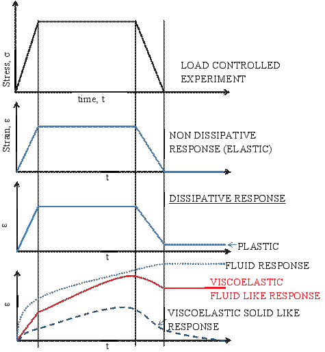
Figure 1.3: Schematic of the variation in the strain with time for various responses when the material is loaded and unloaded.

As mentioned already, in this course we shall focus on the elastic or non-dissipative response only.

 Solution to Boundary Value Problems

A boundary value problem is one in which we specify the traction applied on the surface of a body and/or displacement of the boundary of a body and are interested in finding the displacement and/or the stress at any interior point in the body or on part of the boundary where they were not specified. This specification of the boundary traction and/or displacement is called as boundary condition. The boundary condition is in a sense constitutive relation for the boundary. It tells how the body and its surroundings interact. Thus, in a boundary value problem one needs to prescribe the geometry of the body, the constitutive relation for the material that the body is made up of for the process it is going to be subjected to and the boundary condition. Using this information one needs to find the displacement and stress that the body is subjected to. The so found displacement and stress field should satisfy the equilibrium equations, constitutive relations, compatibility conditions and boundary conditions.

The purpose of formulating and solving a boundary value problem is to:

• To ensure the stresses are within prescribed limits
• To ensure that the displacements are within prescribed limits
• To find the distribution of forces and moments on part of the boundary where displacements are specified

There are four type of boundary conditions. They are

• Displacement boundary condition: Here the displacement of the entire boundary of the body alone is specified. This is also called as Dirichlet boundary condition
• Traction boundary condition: Here the traction on the entire boundary of the body alone is specified. This is also called as Neumann boundary condition
• Mixed boundary condition: Here the displacement is specified on part of the boundary and traction is specified on the remaining part of the boundary. Both traction as well as displacement are not specified over any part of boundary
• Robin boundary condition: Here both the displacement and the traction are specified on the same part of the boundary.

There are three methods by which the displacement and stress field in the body can be found, satisfying all the required governing equations and the boundary conditions. Outline of these methods are presented next. The choice of a method depends on the type of boundary condition.

Displacement method

Here displacement field is taken as the basic unknown. Then, using the strain displacement relation, (1.14) the strain is computed. This strain in substituted in the constitutive relation, (1.17) to obtain the stress. The stress is then substituted in the equilibrium equation (1.6) to obtain 3 second order partial differential equations in terms of the components of the displacement field as,

(1.22)

where Δ(⋅) stands for the Laplace operator and t denotes time. The detail derivation of this equation is given in chapter 7. Equation (1.22) is called the Navier-Lamè equations. Thus, in the displacement method equation (1.22) is solved along with the prescribed boundary condition.

If three dimensional solid elements are used for modeling the body in finite element programs, then the weakened form of equation (1.22) is solved for the specified boundary conditions.

 Stress method

In this method, the stress field is assumed such that it satisfies the equilibrium equations as well as the prescribed traction boundary conditions. For example, in the absence of body forces and static equilibrium, it can be easily seen that if the Cartesian components of the stress are derived from a potential, ϕ =  (x,y,z) called as the Airy’s stress potential as,

(1.23)

then the equilibrium equations are satisfied. Having arrived at the stress, the strain is computed using

(1.24)

obtained by inverting the constitutive relation, (1.17). In order to be able to find a smooth displacement field from this strain, it has to satisfy compatibility condition (1.15). This procedure is formulated in chapter 7 and is followed to solve some boundary value problems in chapters 8 and 9.

 Semi-inverse method

This method is used to solve problems when the constitutive relation is not given by Hooke’s law (1.17). When the constitutive relation is not given by Hooke’s law, displacement method results in three coupled nonlinear partial differential equations for the displacement components which are difficult to solve. Hence, simplifying assumptions are made for the displacement field, wherein a the displacement field is prescribed but for some constants and/or some functions. Except in cases where the constitutive relation is of the form (1.16), one has to make an assumption on the components of the stress which would be nonzero for this prescribed displacement field. Then, these nonzero components of the stress field is found in terms of the constants and unknown functions in the displacement field. On substituting these stress components in the equilibrium equations and boundary conditions, one obtains differential equations for the unknown functions and algebraic equations to find the unknown constants. The prescription of the displacement field is made in such a way that it results in ordinary differential equations governing the form of the unknown functions. Since part displacement and part stress are prescribed it is called semi-inverse method. This method of solving equations would not be illustrated in this course.

Finally, we say that the boundary value problem is well posed if (1) There exist a displacement and stress field that satisfies the boundary conditions and the governing equations (2) There exist only one such displacement and stress field (3) Small changes in the boundary conditions causes only small changes in the displacement and stress fields. The boundary value problem obtained when Hooke’s law (1.17) is used for the constitutive relation is known to be well posed, as will be discussed in chapter 7.